Quiver plots for ggplot2. An extension of ‘ggplot2’ to provide quiver plots to visualise vector fields. This functionality is implemented using a geom to produce a new graphical layer, which allows aesthetic options. This layer can be overlaid on a map to improve visualisation of mapped data.
Installation
The stable version can be installed from CRAN:
install.packages("ggquiver")The development version can be installed from GitHub using:
# install.packages("remotes")
remotes::install_github("mitchelloharawild/ggquiver")
Usage
ggquiver introduces a new geom geom_quiver(), which produces a quiver plot in ggplot2.
Quiver plots for functions can easily be produced using ggplot aeshetics. When a grid is detected, the size of the vectors are automatically adjusted to fit within the grid.
library(ggplot2)
library(ggquiver)
expand.grid(x=seq(0,pi,pi/12), y=seq(0,pi,pi/12)) |>
  ggplot(aes(x=x,y=y,u=cos(x),v=sin(y))) +
  geom_quiver()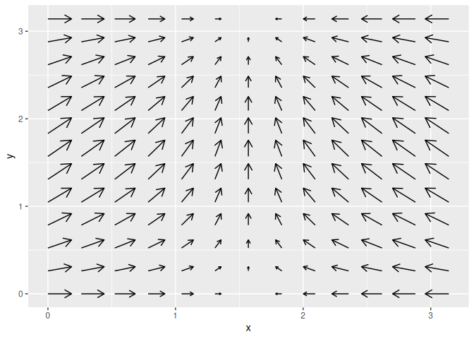
The ggplot2 example for seal movements is easily reproduced, with appropriately scaled arrowhead sizes. Here, the vecsize is set to zero to not resize the vectors.
library(maps)
world <- sf::st_as_sf(map('world', plot = FALSE, fill = TRUE))

ggplot(seals) +
  geom_quiver(
    aes(x=long, y=lat, u=delta_long, v=delta_lat),
    vecsize=0
  ) +
  geom_sf(data = world) +
  coord_sf(xlim = c(-173.8, -117.8), ylim = c(28.7, 50.7), expand = FALSE) +
  labs(title = "Seal movements", x = NULL, y = NULL)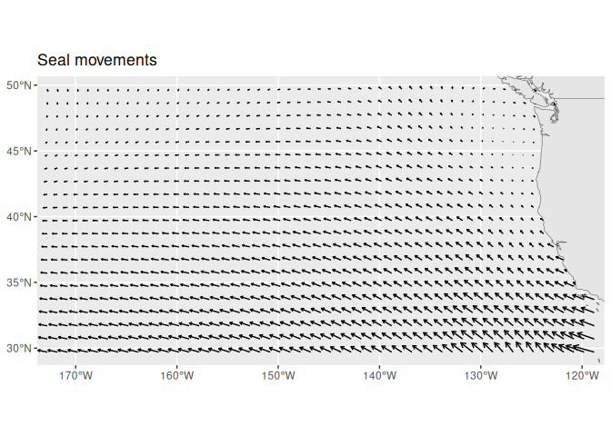
Quiver plot arrows can be centered about x and y coordinates, which is useful when working with maps and scaled vectors.
ggplot(seals) +
  geom_quiver(
    aes(x=long, y=lat, u=delta_long, v=delta_lat),
    vecsize=0, center = TRUE
  ) +
  geom_sf(data = world) +
  coord_sf(xlim = c(-173.8, -117.8), ylim = c(28.7, 50.7), expand = FALSE) +
  labs(title = "Seal movements (centered arrows)", x = NULL, y = NULL)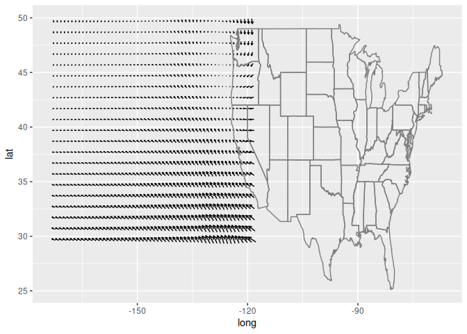
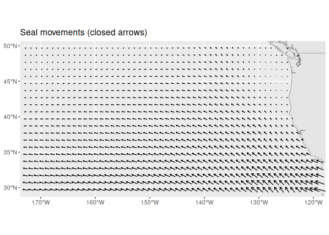
The arrows can be customised using the arrow parameter from grid::arrow(). For example, to use closed arrowheads:
ggplot(seals) +
  geom_quiver(
    aes(x=long, y=lat, u=delta_long, v=delta_lat),
    vecsize=0, center = TRUE,
    arrow = arrow(type = "closed")
  ) +
  geom_sf(data = world) +
  coord_sf(xlim = c(-173.8, -117.8), ylim = c(28.7, 50.7), expand = FALSE) +
  labs(title = "Seal movements (closed arrows)", x = NULL, y = NULL)