Convert a map into a hexagon tile map

Replaces each region of a map with a hexagon of equal size. The hexagons tile the outline of the map, and regions are allocated hexagons by minimising the total squared displacement of all regions (from where the layout moves them), so regions keep their relative positions.

Usage

hexmap(
  object,
  group = NULL,
  layout = layout_hierarchy(),
  island_gap = 0.5,
  group_gap = 0.1,
  crs = NULL
)

Arguments

object: An sf object, or a geometry column (sfc), of regions in a projected or longitude/latitude coordinate reference system.
group: Optionally, the group of each region (e.g. states), as a column of object given unquoted (group = state) or as a string (group = "state"), or as a vector with one value for each region.
layout: How the hexagons (and groups) are arranged, as a layout function such as layout_hierarchy() (the default), layout_diffusion(), layout_compact() or layout_slice(), optionally wrapped in layout_repair() to fix which groups touch.
island_gap: The distance, in hexagon widths, beyond which landmasses are tiled as separate islands. Use Inf to tile all land together.
group_gap: The width of the gap between groups, as a fraction of the hexagon width. The hexagons along group borders are trimmed to make this gap, so they are slightly smaller than other hexagons. Only used with group.
crs: The projected coordinate reference system to make the hexagons in, such as the one the map will be plotted in. object is transformed to crs with sf::st_transform(). Defaults to the CRS of object, or for longitude/latitude input, to a Lambert azimuthal equal-area CRS centred on the data ("+proj=laea +lat_0=... +lon_0=...").

Value

For an sf object, object with its geometry replaced by hexagons, keeping all of its other columns and the order of its rows, so the hexagons can be joined to or compared with the original regions. For a geometry column, a geometry column of hexagons in the same order, so hexmap() can be used within dplyr::mutate() to add the hexagons as another geometry column. The hexagons are in the coordinate reference system they were made in.

Details

Landmasses that are further apart than island_gap hexagon widths are tiled separately, with one hexagon for each region on that landmass. Their hexagons are separated by at least one empty hexagon, so islands such as Tasmania remain distinct from the mainland.

The hexagons are arranged by layout. When group is given, the hexagons of each group (e.g. state) are kept contiguous and a gap of group_gap hexagon widths is cut along the borders between groups, so that each group is visually distinct. Groups usually need a very different area of hexagons than they cover on the map, so the map is distorted to fit them, and each layout distorts it differently. By default, the groups are laid out first, keeping each group's shape and touching the groups it borders on the map, and the regions are then placed within each group. Without group, all regions form a single group, so the layout only sets the shape of the hexagons and where regions are placed within them. See layouts for the available layouts, and vignette("layouts") for how they compare. Grouping works best for groups that are spatially contiguous, such as states.

The hexagons are regular and equally sized in the coordinate reference system (CRS) they are made in, which is the CRS of object unless crs is given, or a Lambert azimuthal equal-area CRS centred on the data for longitude/latitude input. The hexagons keep their location when plotted in another projection, but are stretched by it, so make the hexagons in the CRS you will plot in. Use an equal-area CRS for hexagons that also cover equal areas on the ground. See vignette("projections") for details.

Examples

library(sf)
#> Linking to GEOS 3.12.1, GDAL 3.8.4, PROJ 9.4.0; sf_use_s2() is TRUE
# The 2025 Australian federal election, in the Australian Albers projection
election <- st_transform(aus_election_2025, 3577)
# A hexagon for each electoral division
election_hex <- hexmap(election)

# Every column of the map is kept, in the same order
head(election_hex)
#> Simple feature collection with 6 features and 3 fields
#> Geometry type: POLYGON
#> Dimension:     XY
#> Bounding box:  xmin: -1153976 ymin: -3817828 xmax: 1522580 ymax: -2272518
#> Projected CRS: GDA94 / Australian Albers
#> # A tibble: 6 × 4
#>   division state party                                                  geometry
#>   <chr>    <chr> <chr>                                             <POLYGON [m]>
#> 1 Adelaide SA    ALP   ((-788991 -2553483, -910652.6 -2483242, -910652.6 -23427…
#> 2 Aston    VIC   ALP   ((427625.3 -3396380, 305963.7 -3326138, 305963.7 -318565…
#> 3 Ballarat VIC   ALP   ((-1032314 -3396380, -1153976 -3326138, -1153976 -318565…
#> 4 Banks    NSW   ALP   ((1279257 -3607104, 1157595 -3536863, 1157595 -3396380, …
#> 5 Barker   SA    LP    ((-788991 -2974932, -910652.6 -2904690, -910652.6 -27642…
#> 6 Barton   NSW   ALP   ((1400918 -3817828, 1279257 -3747587, 1279257 -3607104, …

# \donttest{
# Keep the divisions of each state together (takes a few seconds)
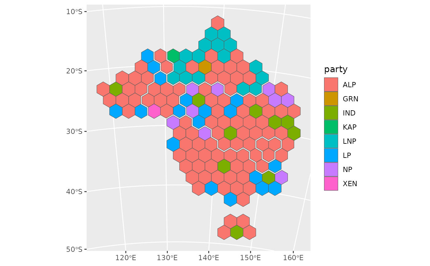
election_hex <- hexmap(election, group = state)
# }

library(ggplot2)
ggplot(election_hex) +
  geom_sf(aes(fill = party))


# \donttest{
# Hexagons made for a globe centred on Australia
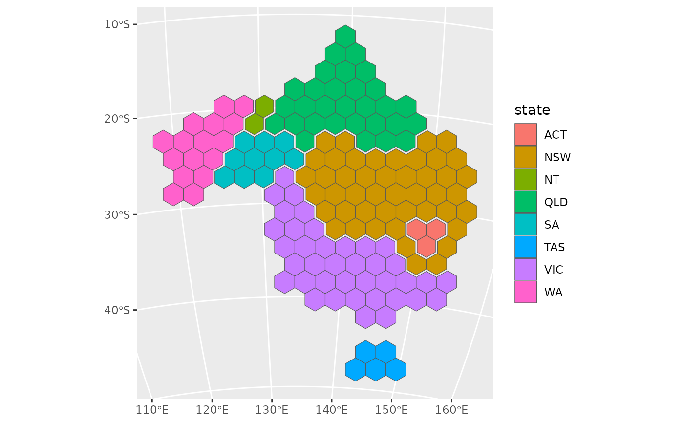
globe <- "+proj=ortho +lat_0=-25 +lon_0=134"
ggplot(hexmap(election, group = state, crs = globe)) +
  geom_sf(aes(fill = state)) +
  coord_sf(crs = globe)

# }
# \donttest{
# Add the hexagons as a second geometry column, alongside the regions
election <- dplyr::mutate(election, hex = hexmap(geometry, group = state))
# }