Line geometry with temporal semantics

geom_time_line() connects observations in order of the time variable, similar to ggplot2::geom_line(), but with special handling for time zones, gaps and duplicated values.

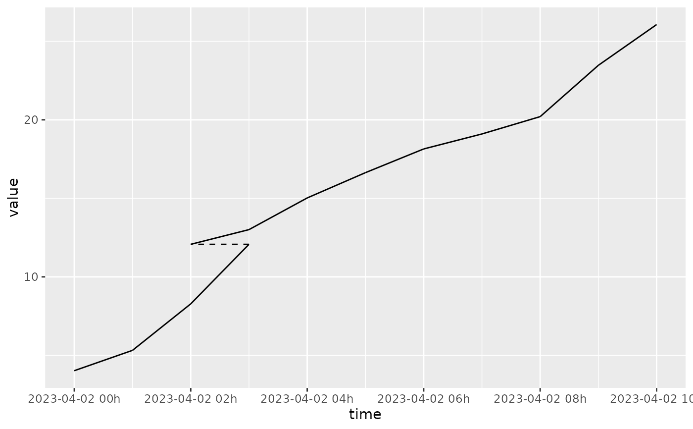
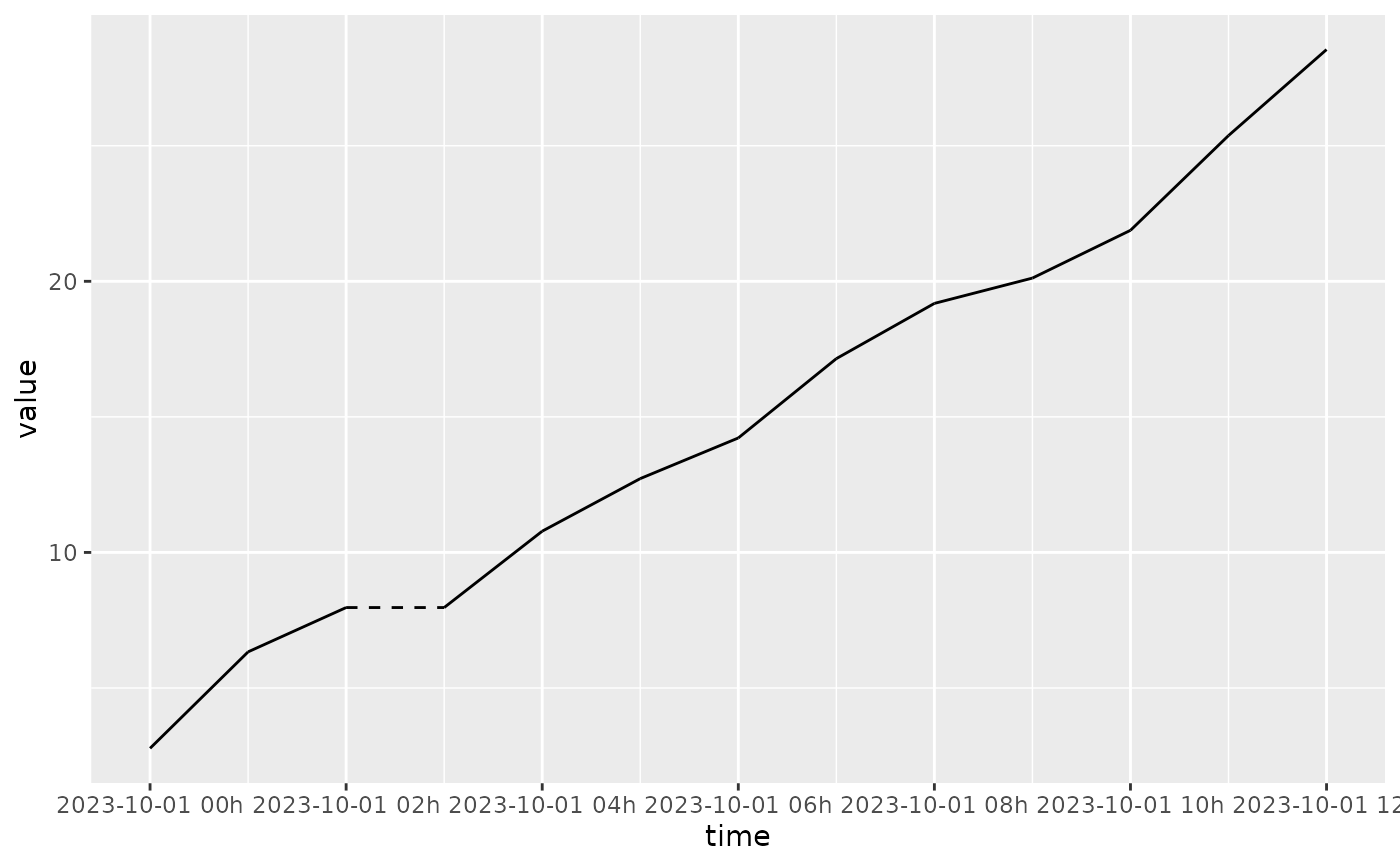
The geometry helps to visualise time with changing time offsets provided by the [x/y]timeoffset aesthetics. Changes in time offsets are drawn using dashed lines, which are most commonly used for timezone changes and daylight savings time transitions. Timezone offsets are automatically used when times from the mixtime package are plotted in local time, which is the scale's default behaviour (see the time_chronon argument of scale_x_mixtime()).

This geometry also respects implicit missing values in regular time series, and will not connect temporal observations separated by gaps.

The ggplot2::group aesthetic determines which cases are connected together.

geom_time_line(
  mapping = NULL,
  data = NULL,
  stat = "identity",
  position = "identity",
  na.rm = FALSE,
  orientation = NA,
  show.legend = NA,
  inherit.aes = TRUE,
  transitions = waiver(),
  transition_aesthetics = list(linetype = 2),
  ...
)

Arguments

mapping

Set of aesthetic mappings created by aes(). If specified and inherit.aes = TRUE (the default), it is combined with the default mapping at the top level of the plot. You must supply mapping if there is no plot mapping.

data

The data to be displayed in this layer. There are three options:

If NULL, the default, the data is inherited from the plot data as specified in the call to ggplot().

A data.frame, or other object, will override the plot data. All objects will be fortified to produce a data frame. See fortify() for which variables will be created.

A function will be called with a single argument, the plot data. The return value must be a data.frame, and will be used as the layer data. A function can be created from a formula (e.g. ~ head(.x, 10)).

stat

The statistical transformation to use on the data for this layer. When using a geom_*() function to construct a layer, the stat argument can be used to override the default coupling between geoms and stats. The stat argument accepts the following:

A Stat ggproto subclass, for example StatCount.
A string naming the stat. To give the stat as a string, strip the function name of the stat_ prefix. For example, to use stat_count(), give the stat as "count".
For more information and other ways to specify the stat, see the layer stat documentation.

position

A position adjustment to use on the data for this layer. This can be used in various ways, including to prevent overplotting and improving the display. The position argument accepts the following:

The result of calling a position function, such as position_jitter(). This method allows for passing extra arguments to the position.
A string naming the position adjustment. To give the position as a string, strip the function name of the position_ prefix. For example, to use position_jitter(), give the position as "jitter".
For more information and other ways to specify the position, see the layer position documentation.

na.rm

If FALSE, the default, missing values are removed with a warning. If TRUE, missing values are silently removed.

orientation

Which positional axis ("x" or "y") carries the time variable that observations are connected in order of. The default (NA) determines this automatically: whichever of x/y is time-valued (a mixtime or POSIXct), preferring x if both (or neither) are.

show.legend

logical. Should this layer be included in the legends? NA, the default, includes if any aesthetics are mapped. FALSE never includes, and TRUE always includes. It can also be a named logical vector to finely select the aesthetics to display. To include legend keys for all levels, even when no data exists, use TRUE. If NA, all levels are shown in legend, but unobserved levels are omitted.

inherit.aes

If FALSE, overrides the default aesthetics, rather than combining with them. This is most useful for helper functions that define both data and aesthetics and shouldn't inherit behaviour from the default plot specification, e.g. annotation_borders().

transitions

A data.frame of known time offset transitions, shaped like mixtime::tz_transitions()'s own output (time a time point, and offset_before/offset_after mixtime::duration()s), with an optional id column to scope rows to a specific series (matched against the xtimeid aesthetic; applied to every series when omitted). Defaults to waiver(), which automatically calls mixtime::tz_transitions() for every timezone present in the data. See the "Time transitions" section below.

transition_aesthetics

A named list of aesthetics for the segment drawn for time transitions, specifying how it is styled differently to the rest of the line. Defaults to list(linetype = 2), drawing transitions with dashed lines. Valid aesthetics are colour/color, linewidth, linetype and alpha.

...

Other arguments passed on to layer()'s params argument. These arguments broadly fall into one of 4 categories below. Notably, further arguments to the position argument, or aesthetics that are required can not be passed through .... Unknown arguments that are not part of the 4 categories below are ignored.

Static aesthetics that are not mapped to a scale, but are at a fixed value and apply to the layer as a whole. For example, colour = "red" or linewidth = 3. The geom's documentation has an Aesthetics section that lists the available options. The 'required' aesthetics cannot be passed on to the params. Please note that while passing unmapped aesthetics as vectors is technically possible, the order and required length is not guaranteed to be parallel to the input data.
When constructing a layer using a stat_*() function, the ... argument can be used to pass on parameters to the geom part of the layer. An example of this is stat_density(geom = "area", outline.type = "both"). The geom's documentation lists which parameters it can accept.
Inversely, when constructing a layer using a geom_*() function, the ... argument can be used to pass on parameters to the stat part of the layer. An example of this is geom_area(stat = "density", adjust = 0.5). The stat's documentation lists which parameters it can accept.
The key_glyph argument of layer() may also be passed on through .... This can be one of the functions described as key glyphs, to change the display of the layer in the legend.

Practical usage

The geom_time_line() geometry extends ggplot2::geom_line() with time semantics that ensure the line's slope accurately reflects rates of change in the measurements over time.

Most notably, geom_time_line() works closely with the time scale (scale_x_mixtime()) to correctly display time in local and absolute time formats. Local time (the scale's default whenever all time points share a timezone) shows time as experienced in that timezone, it is the time on clocks in that timezone. Absolute time shows time as a continuous timeline without timezone adjustments. Which of these is shown is controlled by the scale's time_chronon: a chronon with tz = NA combines time points by their local wall-clock reading (local time), while a chronon with a fixed timezone (such as UTC, the default when a common chronon must be identified across timezones) aligns them by the instant they occurred (absolute time).

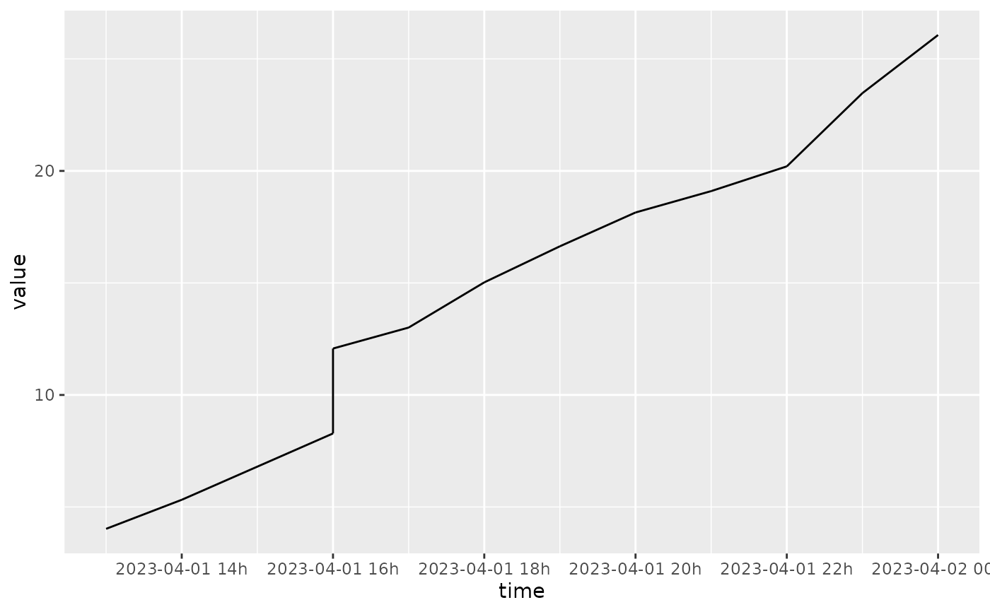
When time series are visualised in local time, timezone offset changes (e.g. due to daylight saving time) cause 'jumps' in time which are indicated with dashed lines. This preserves the integrity of the line's slope across these transitions. Another benefit of visualising time series in local time is to compare time series across different timezones, as the time axis is better aligned with human behaviour in their local timezone (e.g. working hours, sleep patterns, etc). Plotting time series in absolute time shows the exact contemporaneous timing of events across multiple timezones, which is useful when resources or patterns are shared across timezones (e.g. international markets, server load balancing, etc).

This geometry also maintains semantically valid slopes when time values are missing (either implicitly or explicitly), or duplicated. Implicit missing values in regular time series are semantically equivalent to explicit missing values, and geom_time_line() since the slope between unkown values is also unknown, geom_time_line() will not draw lines connecting missing values of either type. Since duplicated time values are not semantically valid in regular time series, geom_time_line() will issue a warning (or an error if systematic duplicates are detected). When drawing a line between duplicated time points, the correct slopes are drawn by connecting all lines that lead to and from the duplicated time points (rather than drawing sawtooth lines).

Further details about each specific capability are described in the following sections.

Time transitions

When time is displayed locally, daylight savings transitions introduce discontinuities in the local timeline when the clock jumps forwards or backwards. geom_time_line() draws these jumps as dashed segments, to preserve the integrity of the line's slope across the transition. When the time scale is set to use local time (see the time_chronon argument of scale_x_mixtime()), the default behaviour (transitions = waiver()) sources daylight savings transitions automatically with mixtime::tz_transitions().

The appearance of transition segments is controlled with transition_aesthetics, a named list of aesthetic overrides (colour, linewidth, linetype and/or alpha). The default is a dashed line.

Offset changes aren't always timezone related. A sensor may be periodically synchronized to adjust for clock drift, or the transitions may reflect an individual's personal travel through time zones. The local time should be mapped to the [x/y] positional aesthetics, with the offset from absolute time mapped to [x/y]timeoffset (a mixtime::duration()). The transitions argument then specifies the instants at which the offset changes, and the offset before and after each transition. This is specified as a data.frame shaped like mixtime::tz_transitions(), with an optional id column to scope rows to a specific series (matched against the [x/y]timeid aesthetic).

Missing time values

Explicit missing values are where an NA value is included in the data, but for regular time series it is also possible to identify implicit missing time values. Unlike ggplot2::geom_line(), geom_time_line() will also not connect points separated by implicit missing values, creating gaps in the line (just like when an explicit missing value is present in ggplot2::geom_line()).

Duplicated time values

If there are duplicated time values within a group, geom_time_line() will issue a warning. An error will be raised if these duplications are systematic across the geometry, specifically if more than 50% of time points contain the same number of duplicates. Systematic duplicates typically indicate a need to use grouping aesthetics (ggplot2::group, or ggplot2::colour) to draw separate lines for each time series. Rather than plotting an erroneous 'sawtooth' line which misrepresents the rate of change, the geometry will draw all lines that connect to and from each of the duplicated time values.

Aesthetics

geom_time_line() understands the following aesthetics. Required aesthetics are displayed in bold and defaults are displayed for optional aesthetics:

•	`x`
•	`y`
•	`alpha`	→ `NA`
•	`colour`	→ via `theme()`
•	`group`	→ inferred
•	`linetype`	→ via `theme()`
•	`linewidth`	→ via `theme()`
•	`xtimeid`
•	`xtimeoffset`
•	`ytimeid`
•	`ytimeoffset`

Learn more about setting these aesthetics in vignette("ggplot2-specs").

Examples


library(ggplot2)


# Basic time line plot of a random walk (no timezone changes)
df_ts <- data.frame(
  time = as.POSIXct("2023-03-11", tz = "Australia/Melbourne") + 0:11 * 3600,
  value = cumsum(rnorm(12, 2))
)
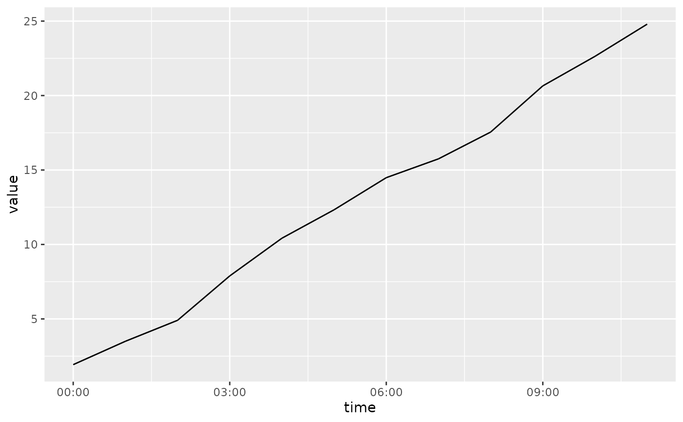
ggplot(df_ts, aes(time, value)) +
  geom_time_line()


# Random walk with a backward timezone change (DST ends)
df_tz_back <- data.frame(
  time = as.POSIXct("2023-04-02", tz = "Australia/Melbourne") + 0:11 * 3600,
  value = cumsum(rnorm(12, 2))
)
# Naive/local time (`tz = NA`) shows the DST transition as a dashed jump
ggplot(df_tz_back, aes(time, value)) +
  geom_time_line() +
  scale_x_mixtime(time_chronon = mixtime::cal_gregorian$hour(1L, tz = NA))

# Absolute time aligns to a single fixed timezone, removing the jump
ggplot(df_tz_back, aes(time, value)) +
  geom_time_line() +
  scale_x_mixtime(time_chronon = mixtime::cal_gregorian$hour(1L, tz = "UTC"))


# Random walk with a forward timezone change (DST starts)
df_tz_forward <- data.frame(
  time = as.POSIXct("2023-10-01", tz = "Australia/Melbourne") + 0:11 * 3600,
  value = cumsum(rnorm(12, 2))
)
ggplot(df_tz_forward, aes(time, value)) +
  geom_time_line() +
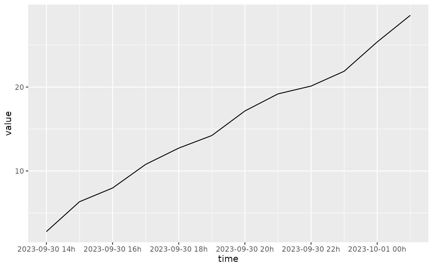
  scale_x_mixtime(time_chronon = mixtime::cal_gregorian$hour(1L, tz = NA))

ggplot(df_tz_forward, aes(time, value)) +
  geom_time_line() +
  scale_x_mixtime(time_chronon = mixtime::cal_gregorian$hour(1L, tz = "UTC"))