Truncate a distribution — dist_truncated • distributional

Note that the samples are generated using inverse transform sampling, and the means and variances are estimated from samples.

dist_truncated(dist, lower = -Inf, upper = Inf)

Arguments

dist: The distribution(s) to truncate.
lower, upper: The range of values to keep from a distribution.

Details

We recommend reading this documentation on pkgdown which renders math nicely. https://pkg.mitchelloharawild.com/distributional/reference/dist_truncated.html

In the following, let $X$ be a truncated random variable with underlying distribution $Y$, truncation bounds lower = $a$ and upper = $b$, where $F_Y(x)$ is the c.d.f. of $Y$ and $f_Y(x)$ is the p.d.f. of $Y$.

Support: $[a, b]$

Mean: For the general case, the mean is approximated numerically. For a truncated Normal distribution with underlying mean $\mu$ and standard deviation $\sigma$, the mean is:

$$ E(X) = \mu + \frac{\phi(\alpha) - \phi(\beta)}{\Phi(\beta) - \Phi(\alpha)} \sigma $$

where $\alpha = (a - \mu)/\sigma$, $\beta = (b - \mu)/\sigma$, $\phi$ is the standard Normal p.d.f., and $\Phi$ is the standard Normal c.d.f.

Variance: Approximated numerically for all distributions.

Probability density function (p.d.f):

$$ f(x) = \begin{cases} \frac{f_Y(x)}{F_Y(b) - F_Y(a)} & \text{if } a \le x \le b \\ 0 & \text{otherwise} \end{cases} $$

Cumulative distribution function (c.d.f):

$$ F(x) = \begin{cases} 0 & \text{if } x < a \\ \frac{F_Y(x) - F_Y(a)}{F_Y(b) - F_Y(a)} & \text{if } a \le x \le b \\ 1 & \text{if } x > b \end{cases} $$

Quantile function:

$$ Q(p) = F_Y^{-1}(F_Y(a) + p(F_Y(b) - F_Y(a))) $$

clamped to the interval $[a, b]$.

Examples

dist <- dist_truncated(dist_normal(2,1), lower = 0)

dist
#> <distribution[1]>
#> [1] N(2, 1)[0,Inf]
mean(dist)
#> [1] 2.055248
variance(dist)
#> [1] 0.8864519

generate(dist, 10)
#> [[1]]
#>  [1] 1.7415534 0.7471783 2.6599636 2.4990165 2.9423018 1.9174482 3.7826920
#>  [8] 1.4461079 3.6731440 1.4203806
#> 

density(dist, 2)
#> [1] 0.4082296
density(dist, 2, log = TRUE)
#> [1] -0.8959256

cdf(dist, 4)
#> [1] 0.9767203

quantile(dist, 0.7)
#> [1] 2.544133

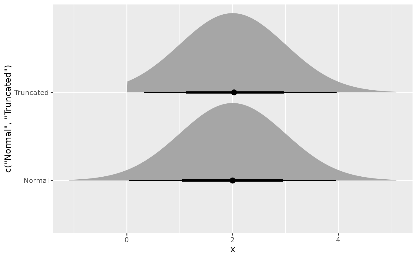
if(requireNamespace("ggdist")) {
library(ggplot2)
ggplot() +
  ggdist::stat_dist_halfeye(
    aes(y = c("Normal", "Truncated"),
        dist = c(dist_normal(2,1), dist_truncated(dist_normal(2,1), lower = 0)))
  )
}